How To Calculate Calibration Curves

Prudence and sound scientific practice require that measuring devices be calibrated. That is, measurements must be carried out on samples with known properties before samples with unknown properties are measured. As an example, consider a thermometer. Just because a thermometer reads 77 degrees Fahrenheit does not mean that the actual temperature in the room is 77 Fahrenheit.

Step 1

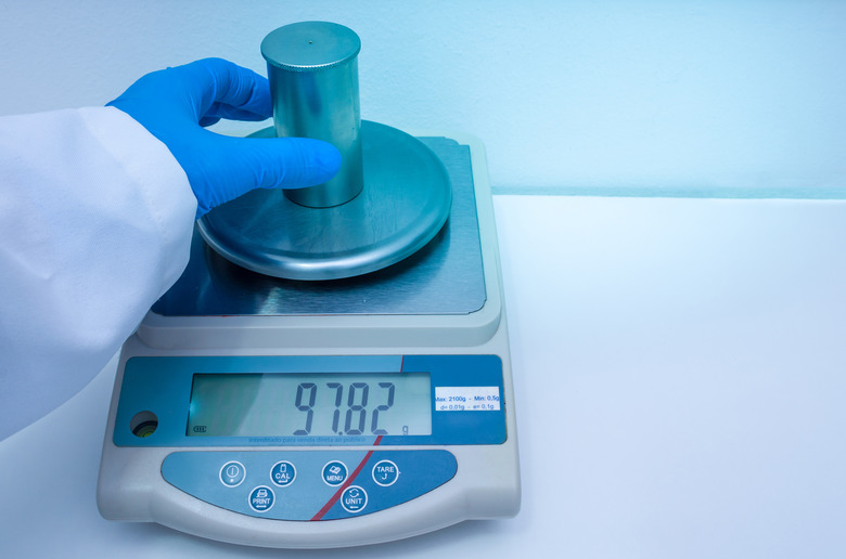
Take at least two measurements of samples with known values. In the case of a thermometer, this may mean immersing the thermometer in ice water (0 degrees Celsius) and in boiling water (100 degrees Celsius). For a balance or set of scales, this would mean measuring weights of known mass, such as 50 grams or 100 grams.

Two such data points are the minimum required, but the old axiom that "more is better" holds true.

Step 2

Construct a graph of the calibration measurements by plotting the "known" value on the y-axis and the "experimental" value on the x-axis. This can be done manually (i.e., by hand on graph paper) or with the aid of a computer graphing program, such as Microsoft Excel or OpenOffice Calc. Purdue University offers a brief tutorial on graphing with Excel. The University of Delaware offers a similar guide for Calc.

Draw a straight line through the data points and determine the equation of the line (most computer graphing programs refer to this as "linear regression"). The equation will be of the general form y = mx + b, where m is the slope and b is the y-intercept, such as y = 1.05x + 0.2.

Step 3

Use the equation of the calibration curve to adjust measurements taken on samples with unknown values. Substitute the measured value as x into the equation and solve for y (the "true" value). In the example from step 2, y = 1.05x + 0.2. Thus, a measured value of 75.0, for example, would adjust to y = 1.05(75) + 0.2 = 78.9.