How To Use A Graphing Calculator

A graphing calculator is a standard tool for high school level math courses like algebra, precalculus, calculus, and trigonometry. Learning how to use one properly is essential for these classes, not to mention its many uses in the fields of science and engineering. A graphing calculator is a specific type of scientific calculator that includes a screen on which you can graph mathematical functions. There are multiple brands and models of graphic calculators, with the best-selling being Texas Instruments' TI-84 models, which our instructions will be based on. Most graphing calculators have the same basic operation as this model, but it is still important to read the instructions for your specific calculator.

A graphing calculator has a few different components to its interface. At the top is the screen on which all of your graphs and equations will be displayed. Below that is a keypad, which includes all the familiar parts of any basic calculator. However, it also includes some extra components. There is an arrow keypad for navigating the graph and menus (using the "enter" button to choose menu options), as well as a series of graphing keys. 

One thing to note is that most of the keys on a graphing calculator have more than one function. In addition to the label on the key itself, you should see one or two additional labels written above. You can switch to these functions by using the "2nd" and "ALPHA" keys, which work like the "Shift" button on a computer keyboard. With that out of the way, let's talk about graphing functions.

Directly beneath the screen on your graphing calculator is a row of five graphing keys: "Y," which allows you to enter an equation to graph; "WINDOW," to adjust the axes of the graph; "ZOOM," for zooming in or out of graphs; "TRACE," which switches to a cursor that you can use to navigate the graph, and "GRAPH,"  which converts functions into a graph.

Graphing calculators only work on functions with two variables: x and y. In order to graph equations, you need them to be in the form of y=, so if you were trying to graph the equation x+y=5, you'd first need to convert it to y=5-x. Once you have your equation in the form of y=, enter it into the calculator using the "y=" key. Use the "X, T, ϴ, n" key to enter the variable x. If your equation has any exponents, use the "E" key on your calculator.

The next step is to set the boundaries of your graph. Press "WINDOW," then use the "Xmin" and "Xmax" keys to set the x axis of the graph and the "Ymin" and "Ymax" keys to set the y axis. Finally, press the "GRAPH" key to generate your graph. Although base models of graphing calculators require you to graph y in terms of x, you can graph x in terms of y on a TI-84 calculator by downloading additional software.

Regression analysis is used to determine the relationship between a single dependent variable and one or more independent variables. The most common kind of regression is linear regression, which is plotted on a graph in a straight line.

To calculate linear regression on your graphing calculator, begin by pressing the "STAT" key and select "EDIT" (which should already be highlighted as the first option) by pressing "enter." This will open a screen with a series of columns numbered L1, L2, L3, and so on, which you can select using the arrow keypad. Enter your x values in the L1 column and your y values in L2, pressing "enter" after each number. Quit the screen by pressing the "2nd" then the "mode" ("quit") buttons (your data will be saved) and press "STAT" again, this time selecting the "CALC" menu by using the right arrow button. Scroll down to the option "LinReg (ax+b)" and select it. Now, press the "2nd" and "1" keys, followed by a comma, then the "2nd" and "2", which will load the data you previously entered in the L1 and L2 columns. Scroll down to "calculate" and press "enter" to determine the regression values.

To plot a linear regression, press the "2nd" key followed by the "y=" key, which will open the "Stat Plots" menu. Select "Plot 1" and choose the scatter plot option. Set the Xlist to "L1" and the Ylist to "L2" to load the x and y values you previously entered. Finally, press the "GRAPH" key to generate your scatter plot. If you return to the "LinReg" screen, you'll see values for a and b for a y=ax+b equation, and pressing "GRAPH" will generate the line of best fit on your scatter plot.

The second type of regression is non-linear regression, which is plotted on a curved line. Non-linear regressions are often used to analyze growth patterns, such as exponential growth, in which one factor grows at an increasing rate in response to another factor, and logarithmic growth, in which one factor grows at a decreasing rate in response to the other factor. Non-linear regressions are therefore very useful when measuring population changes.

Creating a non-linear regression model on a graphing calculator starts with the same steps used for linear regressions. Press the "STAT" key and select the "EDIT" option. Once again, you'll need to enter your x values into the L1 column and your y values in the L2 column. Use the "Stat Plots" function to generate a scatter plot, just as with a linear regression.

From the scatter plot, you'll need to determine what kind of non-linear regression fits the data (exponential, logarithmic, etc.). Once you've figured that out, press "STAT" and select "CALC," but instead of selecting the "LinReg" option, choose the option that fits your regression type (for example, exponential regression is "ExpReg"). Set the Xlist and Ylist to L1 and L2 respectively, and scroll down to "StoreRegEQ". Next, press the "VARS" key, choose "Y-VARS," select the function you want, and press "enter." Then select "Calculate" to generate the regression in equation form. Finally, press "GRAPH" to create the line of best fit over your scatter plot.

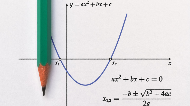
Quadratic equations take the form: ax²+bx+c=0, requiring you to find the value of the variable x. It's also important to note that, in quadratic equations, the value of a can never be zero. When graphed, all quadratic equations take the form of a parabola. If the parabola opens downward, then the vertex (the peak of the curve) represents the function's maximum value, and if the parabola opens upwards, the vertex represents the minimum value.

To create one of these parabolic graphs, start by pressing the "y=" button on your calculator. Use y in place of zero, leaving you with an equation in the form of y=ax²+bx+c. Then, press the "GRAPH" key to generate your graph. Make sure it takes the form of a parabola; you may need to adjust the window using the "ZOOM" key in order to get the proper shape in view.

To find the vertex of the parabola, press the "2nd" key followed by the "TRACE" key, which will open the calculate menu. This allows you to choose whether the vertex is a maximum or minimum. Select the appropriate option, then press "ENTER". Define the left and right bounds by using the left and right arrows on the keypad. Press "ENTER" one more time to calculate the coordinates of the vertex. To find the x-intercepts, open the calculate menu again and select zero. Then repeat the steps you used to find the vertex.